Tutorial¶

In this tutorial we show a step-by-step application of HEMDAG to the hierarchical prediction of associations between human gene and abnormal phenotype. To this end we will use the small pre-built dataset available in the HEMDAG library. However, all the hierarchical ensemble methods encompassed in HEMDAG library can be run by using:

any ontology listed in OBO foundry (link);

any flat score matrix, achieved by using any flat classifier ranging from linear, to probabilistic methods, to neural networks, to gradient boosting and many others;

any annotation matrix.

Of course, the number of terms among the graph, the flat score matrix and the annotation matrix must match.

Note

To run the experiments shown in this page, make sure you have installed the following requirements:

HEMDAG >= 2.7.4

R >= 3.4.4

Ubuntu >= 16.04

Load the HEMDAG Library¶

To load the HEMDAG library, open the R environment and type:

library(HEMDAG);

Load the Flat Scores Matrix¶

In their more general form, the hierarchical ensemble methods adopt a two-step learning strategy:

the first step consists in the flat learning of the ontology terms;

the second step reconciles the flat predictions by considering the topology of the underlying ontology.

Consequently, the first ingredient that we need in a hierarchical ensemble classification is the flat score matrix. For the sake of simplicity, in the examples shown below we use the pre-built dataset available in the HEMDAG library. To load the flat score matrix, type in the the R environment:

data(scores);

With the above command we loaded the flat score matrix S, that is a named 100 X 23 matrix. Rows correspond to genes (Entrez GeneID) and columns to HPO terms/classes. The scores represent the likelihood that a given gene belongs to a given class: the higher the value, the higher the likelihood that a gene belongs to a given class. This flat score matrix was obtained by running the RANKS package (link).

Normalization¶

Since RANKS returns a score and not a probability, we must normalize the scores of the matrix S to make the flat scores comparable with the hierarchical ones. In case the flat classifier returns directly a probability there is no needed to normalize the flat score matrix, since the flat scores can be directly compared with the hierarchical ones.

HEMDAG allows to normalize the flat scores according to two different procedures:

maxnorm: Normalization in the sense of the maximum: the score of each class is normalized by dividing the score values for the maximum score of that class:

S.maxnorm <- scores.normalization(norm.type="maxnorm", S);

qnorm: Quantile normalization: quantile normalization of the preprocessCore package is used:

S.qnorm <- scores.normalization(norm.type="qnorm", S);

Be sure to install the preprocessCore package before running the above command. Yo can install it by conda (conda install -c bioconda bioconductor-preprocesscore) or by Bioconductor (link)

Note

For the sake of simplicity, in all the examples shown in section Hierarchical Ensemble Methods, the input flat score matrix was normalized according to the maxnorm normalization:

S.norm <- scores.normalization(norm.type="maxnorm", S);

Load the Graph¶

In order to know how the hierarchical structure of the HPO terms, we need to load the graph:

data(graph);

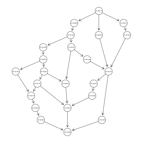
With the above command we loaded the graph g, an object of class graphNEL. The graph g has 23 nodes and 30 edges and represents the ancestors view of the HPO term Camptodactyly of finger (HP:0100490). Nodes of the graph g correspond to terms of the flat score matrix S.

Plot the Graph (optional)¶

Note

To plot the graph you need to install before the Rgraphviz package. Yo can install this library for example by conda (conda install -c bioconda bioconductor-rgraphviz) or by Bioconductor (link).

If you want to visualize the ancestors view of the term HP:0100490, just type:

library(Rgraphviz);
plot(g);

Utility Functions for Graphs (optional)¶

HEMDAG includes 33 utility functions (listed below) to process and analyze graphs as well as I/O functions to import a graph as object of class graphNEL or to export a graph as object of class graphNEL in a plain text file (in the classical tupla format). For more details on these functions, refer to the reference manual.

build.ancestors                         build.parents                              constraints.matrix
build.ancestors.bottom.up               build.parents.bottom.up                    distances.from.leaves
build.ancestors.per.level               build.parents.top.down                     find.leaves
build.children                          build.parents.topological.sorting          graph.levels
build.children.bottom.up                build.scores.matrix.from.list              lexicographical.topological.sort
build.children.top.down                 build.scores.matrix.from.tupla             read.graph
build.consistent.graph                  build.subgraph                             read.undirected.graph
build.descendants                       check.dag.integrity                        root.node
build.descendants.bottom.up             check.hierarchy                            tupla.matrix
build.descendants.per.level             check.hierarchy.single.sample              weighted.adjacency.matrix
build.edges.from.hpo.obo                compute.flipped.graph                      write.graph

Hierarchical Ensemble Methods¶

First of all, we need to find the root node (i.e. node that is at the top-level of the hierarchy) of the HPO graph g. To do that just type:

root <- root.node(g);

in this way we store in the variable root the root node of the graph g.

Now, we are ready to run any ensemble algorithms implemented in the HEMDAG package.

HTD-DAG: Hierarchical Top Down for DAG¶

The HTD-DAG algorithm modifies the flat scores according to the hierarchy of a DAG \(G\) through a unique run across the nodes of the graph. For a given example \(x\), the flat predictions \(f(x) = \hat{y}\) are hierarchically corrected to \(\bar{y}\), by per-level visiting the nodes of the DAG from top to bottom according to the following simple rule:

\[\begin{split}\bar{y}_i := \left\{ \begin{array}{lll} \hat{y}_i & {\rm if} \quad i \in root(G) \\ \min_{j \in par(i)} \bar{y}_j & {\rm if} \quad \min_{j \in par(i)} \bar{y}_j < \hat{y}_i \\ \hat{y}_i & {\rm otherwise} \end{array} \right.\end{split}\]

The node levels correspond to their maximum path length from the root. To call the HTD-DAG algorithm just type:

S.htd <- htd(S.norm, g, root);

Alternatively, we can call the htd.vanilla function (instead of htd), which it allows to normalize the flat score matrix S (according to maxnorm or qnorm normalization) on the fly:

run a normalization method (between maxnorm and qnrom) on the fly:

S.htd <- htd.vanilla(S, g, norm=TRUE, norm.type="maxnorm");

Note

In htd.vanilla, if norm=FALSE and norm.type=NULL the flat score matrix S is not normalized.

GPAV: Generalized Pool-Adjacent-Violators¶

Burdakov et al. in [1] proposed an approximate algorithm, named GPAV, to solve the isotonic regression (IR) or monotonic regression (MR) problem in its general case (i.e. partial order of the constraints). GPAV algorithm combines both low computational complexity (estimated to be \(\mathcal{O}(|V|^2\)), where \(V\) is the number of nodes of the graph) and high accuracy. Formally, given a vector of observed values \(\hat{y} \in R^n\), a strictly positive vector of weights \(w \in R^n\) and a dag \(G(V,E)\), GPAV finds the vector of fitted values \(\bar{y} \in \mathbb{R}^n\) that solves the following convex quadratic program:

\[\begin{split}\begin{equation} \begin{array}{ll} \min\limits_{\bar{y}} \quad \sum\limits_{i \in V} w_i (\bar{y}_i - \hat{y}_i)^2 \\ s.t. \quad \bar{y}_j \geq \bar{y}_i \quad \forall (i,j) \in E \end{array} \end{equation}\end{split}\]

To call the GPAV algorithm just type:

S.gpav <- gpav.over.examples(S.norm, g, W=NULL);

It is worth noting that there is also a parallel version of the GPAV algorithm:

S.gpav <- gpav.parallel(S.norm, g, W=NULL, ncores=8);

Similarly to HTD-DAG also for GPAV, we can use the function gpav.vanilla (instead of gpav.over.examples or gpav.parallel) to normalize the flat score matrix S (according to maxnorm or qnorm normalization) on the fly:

S.gpav <- gpav.vanilla(S, g, W=NULL, parallel=TRUE, ncores=8, norm=TRUE, norm.type="maxnorm");

TPR-DAG: True Path Rule for DAG¶

TPR-DAG is a family of algorithms on the basis of the choice of the bottom-up step adopted for the selection of positive children. Indeed, in their more general form, the TPR-DAG algorithms adopt a two step learning strategy:

in the first step they compute a per-level bottom-up visit from leaves to root to propagate positive predictions across the hierarchy;

in the second step they compute a per-level top-down visit from root to leaves in order to assure the consistency of the predictions. In other word, the HTD-DAG: Hierarchical Top Down for DAG algorithm is applied.

Note

Levels (both in the first and second step) are defined in terms of the maximum path length from the root node. Please refer to [3] for further details.

The vanilla TPR-DAG adopts a per-level bottom-up traversal of the DAG to modify the flat predictions \(\hat{y}_i\) according to the following formula:

\[\bar{y}_i := \frac{1}{1 + |\phi_i|} (\hat{y}_i + \sum_{j \in \phi_i} \bar{y}_j)\]

where \(\phi_i\) are the positive children of \(i\) (parameter positive="children").

Different strategies to select the positive children \(\phi_i\) can be applied:

threshold-free strategy (parameter bottom="threshold.free"): the positive nodes are those children that can increment the score of the node \(i\), that is those nodes that achieve a score higher than that of their parents:

\[\phi_i := \{ j \in child(i) | \bar{y}_j > \hat{y}_i \}\]

threshold strategy (parameter bottom="threshold"): the positive children are selected on the basis of a threshold that can be selected in two different ways:

a unique threshold \(\bar{t}\) is a priori selected for all nodes to determine the set of positives

\[\phi_i := \{ j \in child(i) | \bar{y}_j > \bar{t} \}, \forall i \in V\]

For instance if the predictions represent probabilities it could be meaningful set \(\bar{t}=0.5\).

a threshold is selected to maximize some imbalance-aware performance metric \(\mathcal{M}\) estimated on the training data, as for instance the Fmax or the AUPRC. In other words, the threshold is selected to maximize the measure \(\mathcal{M}(j,t)\) on the training data for the term \(j\) with respect to the threshold \(t\). The corresponding set of positives for each \(i \in V\) is:

\[\phi_i := \{ j \in child(i) | \bar{y}_j > t_j^*, t_j^* = \arg \max_{t} \mathcal{M}(j,t) \}\]

Internal cross-validation is used to select \(t^*_j\) within a set of possible thresholds \(t \in (0,1)\);

The weighted TPR-DAG version (parameter bottom="weighted.threshold.free") can be designed by adding a weight \(w \in [0,1]\) to balance the contribution of the parent node \(i\) and its positive children \(\phi\):

\[\bar{y}_i := w \hat{y}_i + \frac{(1 - w)}{|\phi_i|} \sum_{j \in \phi_i} \bar{y}_j\]

If \(w=1\) no weight is attributed to the children and the TPR-DAG reduces to the HTD-DAG algorithm. If \(w=0\) only the predictors associated to the children nodes vote to predict node \(i\). In the intermediate cases we attribute more importance to the predictor for the node \(i\) or to its children depending on the values of \(w\).

By combining the weighted and the threshold variant, we design the weighted-threshold variant (parameter bottom="weighted.threshold").

All the vanilla TPR-DAG variants use the HTD-DAG algorithm in the top-down step (parameter topdown="htd") to provide ontology-based predictions (i.e. predictions that are coherent with the ontology structure):

S.tprTF <- tpr.dag(S.norm, g, root, positive="children", bottomup="threshold.free", topdown="htd");
S.tprT  <- tpr.dag(S.norm, g, root, positive="children", bottomup="threshold", topdown="htd", t=0.5);
S.tprW  <- tpr.dag(S.norm, g, root, positive="children", bottomup="weighted.threshold.free", topdown="htd", w=0.5);
S.tprWT <- tpr.dag(S.norm, g, root, positive="children", bottomup="weighted.threshold", topdown="htd", t=0.5, w=0.5);

DESCENS: Descendants Ensemble Classifier¶

As shown in [5] for tree-based hierarchies, the contribution of the descendants of a given node decays exponentially with their distance from the node itself and it is straightforward to see that this property also holds for DAG structured taxonomies. To overcame this limitation and in order to enhance the contribution of the most specific nodes to the overall decision of the ensemble we design the ensemble variant DESCENS. The novelty of DESCENS consists in strongly considering the contribution of all the descendants of each node instead of only that of its children (positive="descendants"). Therefore DESCENS predictions are more influenced by the information embedded in the leaves nodes, that are the classes containing the most informative and meaningful information from a biological and medical standpoint. DESCENS variants can be designed on the choice of the positive descendants \(\Delta_i\). The same strategies adopted for the choice of \(\phi_i\) can be also adopted for the choice of \(\Delta_i\), simply by replacing \(\phi_i\) with \(\Delta_i\) and \(child(i)\) with \(desc(i)\) in the various formulas shown in TPR-DAG: True Path Rule for DAG. Furthermore, we designed a variant specific only for DESCENS, that we named DESCENS-\(\tau\) (parameter bottomup="tau"). The DESCENS-\(\tau\) variant balances the contribution between the positives children of a node \(i\) and that of its positives descendants excluding its children by adding a weight \(\tau \in [0,1]\):

\[\bar{y}_i := \frac{\tau}{1+|\phi_i|}(\hat{y}_i + \sum_{j \in \phi_i} \bar{y}_j) + \frac{1-\tau}{1+|\delta_i|}(\hat{y}_i + \sum_{j\in \delta_i} \bar{y}_j)\]

where \(\phi_i\) are the positive children of \(i\) and \(\delta_i=\Delta_i \setminus \phi_i\) the descendants of \(i\) without its children.

If \(\tau=1\) we consider only the contribution of the positive children of \(i\); if \(\tau=0\) only the descendants that are not children contribute to the score, while for intermediate values of \(\tau\) we can balance the contribution of \(\phi_i\) and \(\delta_i\) positive nodes.

All the DESCENS variants adopt in the second step the HTD-DAG algorithm to assure the consistency of the predictions:

S.descensTF  <- tpr.dag(S.norm, g, root, positive="descendants", bottomup="threshold.free", topdown="htd");
S.descensT   <- tpr.dag(S.norm, g, root, positive="descendants", bottomup="threshold", topdown="htd", t=0.5);
S.descensW   <- tpr.dag(S.norm, g, root, positive="descendants", bottomup="weighted.threshold.free", topdown="htd", w=0.5);
S.descensWT  <- tpr.dag(S.norm, g, root, positive="descendants", bottomup="weighted.threshold", topdown="htd", t=0.5, w=05);
S.descensTAU <- tpr.dag(S.norm, g, root, positive="descendants", bottomup="tau", topdown="htd", t=0.5);

ISO-TPR: Isotonic Regression for DAG¶

The ISO-TPR algorithms (parameter positive="children" and topdown="gpav") considering the positive children in the bottom-up step and adopt GPAV (GPAV: Generalized Pool-Adjacent-Violators) instead of HTD-DAG (HTD-DAG: Hierarchical Top Down for DAG) in the consistency step. The most important feature of the ISO-TPR algorithms is that they maintain the hierarchical constraints by construction by selecting the closest solution (in the least square sense) to the bottom-up predictions that obey the True Path Rule:

S.isotprTF <- tpr.dag(S.norm, g, root, positive="children", bottomup="threshold.free", topdown="gpav");
S.isotprT  <- tpr.dag(S.norm, g, root, positive="children", bottomup="threshold", topdown="gpav", t=0.5);
S.isotprW  <- tpr.dag(S.norm, g, root, positive="children", bottomup="weighted.threshold.free", topdown="gpav", w=0.5);
S.isotprWT <- tpr.dag(S.norm, g, root, positive="children", bottomup="weighted.threshold", topdown="gpav", t=0.5, w=0.5);

ISO-DESCENS: Isotonic Regression with Descendants Ensemble Classifier¶

The ISO-DESCENS variants (parameter positive="descendants" and topdown="gpav") considering the positive descendants instead of positive children in the bottom-up step and adopt GPAV (instead of the HTD-DAG algorithm) to guarantee the consistency of the predictions:

S.isodescensTF  <- tpr.dag(S.norm, g, root, positive="descendants", bottomup="threshold.free", topdown="gpav");
S.isodescensT   <- tpr.dag(S.norm, g, root, positive="descendants", bottomup="threshold", topdown="gpav", t=0.5);
S.isodescensW   <- tpr.dag(S.norm, g, root, positive="descendants", bottomup="weighted.threshold.free", topdown="gpav", w=0.5);
S.isodescensWT  <- tpr.dag(S.norm, g, root, positive="descendants", bottomup="weighted.threshold", topdown="gpav", t=0.5, w=0.5);
S.isodescensTAU <- tpr.dag(S.norm, g, root, positive="descendants", bottomup="tau", topdown="gpav", t=0.5);

Obozinski Heuristic Methods¶

HEMDAG includes also the three heuristics ensemble methods (And, Max, Or) proposed in [4]:

Max: reports the largest logistic regression (LR) value of self and all descendants: \(p_i = max_{j \in descendants(i)} \hat{p_j}\);
And: reports the product of LR values of all ancestors and self. This is equivalent to computing the probability that all ancestral terms are “on” assuming that, conditional on the data, all predictions are independent: \(p_i = \prod_{j \in ancestors(i)} \hat{p_j}\);
Or: computes the probability that at least one of the descendant terms is “on” assuming again that, conditional on the data, all predictions are independent: \(1 - p_i = \prod_{j \in descendants(i)} (1 - \hat{p_j})\);

To call Obozinski’s heuristic methods, just type:

S.max <- obozinski.max(S.norm, g, root);
S.and <- obozinski.and(S.norm, g, root);
S.or  <- obozinski.or(S.norm, g, root);

Alternatively, the Obozinski’s methods can be also called by properly setting the parameter heuristic of the function obozinski.methods:

S.max <- obozinski.methods(S, g, heuristic="max", norm=TRUE, norm.type="maxnorm");
S.and <- obozinski.methods(S, g, heuristic="and", norm=TRUE, norm.type="maxnorm");
S.or  <- obozinski.methods(S, g, heuristic="or",  norm=TRUE, norm.type="maxnorm");

Check Hierarchical Constraints¶

Predictions returned by a flat classifier do not respect the True Path Rule (since they neglect the structural information between different ontology terms), whereas the predictions returned by a hierarchical ensemble methods always obey the True Path Rule. According to this rule a positive instance for a class implies positive instance for all the ancestors of that class. We can easily check this fact by using the function check.hierarchy. Below (as an example) we check the consistency of the scores corrected according to the HTD-DAG strategy. Of course, all the scores matrices corrected with any hierarchical ensemble variants included in HEMDAG, respect the True Path Rule. We leave to the user the freedom to check the consistency of the scores matrix of the remaining 22 hierarchical ensemble variants encompassed in HEMDAG.

check.hierarchy(S, g, root)$status
"NOTOK"

check.hierarchy(S.htd, g, root)$status
"OK"

Performance Evaluation¶

To know the behavior of the hierarchical ensemble methods, the HEMDAG library provides both term-centric and protein-centric performance metrics:

AUPRC: area under the precision-recall curve;
AUROC: area under the ROC curve;
Fmax : maximum hierarchical F-score [2];
PXR : precision at different recall levels;

Note

HEMDAG allows to compute all the aforementioned performance metrics either one-shot or averaged across k fold. Depending on the dataset size, the metrics Fmax and PXR could take a while to finish. Please refer to HEMDAG reference manual for further information about the input arguments of these functions.
For computing the term-centric metrics (AUROC, AUPRC and PXR), HEMDAG makes use of the R package precrec (link).

Load the Annotation Matrix¶

To compare the hierarchical ensemble methods against the flat approach, we need to load the annotation matrix:

data(labels);

With the above command we loaded the annotations table L, that is a named 100 X 23 matrix. Rows correspond to genes (Entrez GeneID) and columns to HPO terms/classes. L[i, j] = 1 means that the gene i belong to class j, L[i, j] = 0 means that the gene i does not belong to class j.

Flat vs Hierarchical¶

Before computing performance metrics we should remove the root node from the annotation matrix, the flat score matrix and the hierarchical scores matrix. Indeed, it does not make sense to take into account the predictions of the root node, since it is a fake node added to the ontology for practical reasons (e.g. some graph-based software may require a single root node to work). In R this can be accomplished in one line of code.

## remove root node from annotation matrix
if(root %in% colnames(L))
    L <- L[,-which(colnames(L)==root)];

## remove root node from the normalized flat score matrix
if(root %in% colnames(S.norm))
    S.norm <- S.norm[,-which(colnames(S.norm)==root)];

## remove root node from hierarchical scores matrix (eg S.htd)
if(root %in% colnames(S.htd))
    S.htd <- S.htd[,-which(colnames(S.htd)==root)];

Now we can compare the flat approach RANKS versus the HTD-DAG strategy, by averaging (for instance) the performance across 3 folds:

## RANKS
prc.flat  <- auprc.single.over.classes(L, S.norm, folds=3, seed=23);
auc.flat  <- auroc.single.over.classes(L, S.norm, folds=3, seed=23);
pxr.flat  <- precision.at.given.recall.levels.over.classes(L, S.norm, recall.levels=seq(from=0.1, to=1, by=0.1), folds=3, seed=23);
fmax.flat <- compute.fmax(L, S.norm, n.round=3, verbose=FALSE, b.per.example=TRUE, folds=3, seed=23);

## HTD-DAG
prc.htd  <- auprc.single.over.classes(L, S.htd, folds=3, seed=23);
auc.htd  <- auroc.single.over.classes(L, S.htd, folds=3, seed=23);
pxr.htd  <- precision.at.given.recall.levels.over.classes(L, S.htd, recall.levels=seq(from=0.1, to=1, by=0.1), folds=3, seed=23);
fmax.htd <- compute.fmax(L, S.htd, n.round=3, verbose=FALSE, b.per.example=TRUE, folds=3, seed=23);

By looking at the results, it easy to see that the HTD-DAG outperforms the flat classifier RANKS:

## AUC performance: RANKS VS HTD-DAG
auc.flat$average
0.8297
auc.htd$average
0.8336

## PRC performance: RANKS VS HTD-DAG
prc.flat$average
0.4333
prc.htd$average
0.4627

## Fmax performance: RANKS VS HTD-DAG
fmax.flat$average
    P      R      S      F    avF      A      T
0.5042 0.8639 0.4485 0.6368 0.5269 0.6612 0.5720
fmax.htd$average
    P      R      S      F    avF      A      T
0.5576 0.7745 0.6519 0.6484 0.5617 0.7521 0.6487

## PXR: RANKS VS HTD-DAG
pxr.flat$average
   0.1    0.2    0.3    0.4    0.5    0.6    0.7    0.8    0.9    1
0.5821 0.5821 0.5821 0.5531 0.5531 0.4483 0.4388 0.4388 0.4388 0.4388
pxr.htd$average
   0.1    0.2    0.3    0.4    0.5    0.6    0.7    0.8    0.9    1
0.6218 0.6218 0.6218 0.5941 0.5941 0.4798 0.4668 0.4668 0.4668 0.4668

Note

HTD-DAG is the simplest ensemble approach among those available. HTD-DAG strategy makes flat scores consistent with the hierarchy by propagating from top to bottom the negative predictions. Hence, in the worst case might happen that the predictions at leaves nodes are all negatives. Other ensemble algorithms, such as GPAV and TPR-DAG (and variants) should lead to better improvements.

Tuning of Hyper-Parameter(s)¶

14 out of 18 of the TPR-DAG hierarchical algorithms are parametric. Instead of use a fixed threshold (as done in TPR-DAG: True Path Rule for DAG), we can tune the hyper-parameter(s) of the parametric variants through the function tpr.dag.cv. The hyper-parameter(s) can be maximize on the basis of AUPRC (parameter metric="prc") or Fmax (parameter metric="fmax"). Below, as an example, we maximize the threshold of the parametric variant isotprT on the basis of AUPRC metric.

threshold <- seq(0.1, 0.9, 0.1);

S.isotprT <- tpr.dag.cv(S, g, ann=L, norm=TRUE, norm.type="maxnorm", positive="children",
                        bottomup="threshold", topdown="gpav", W=NULL, parallel=FALSE,
                        ncores=1, threshold=threshold, weight=0, kk=3, seed=23,
                        metric="auprc", n.round=NULL);

## stdout
maxnorm normalization: done
training fold:  1   top auprc avg found:    0.4743567   best threshold: 0.1
training fold:  1   top auprc avg found:    0.4883769   best threshold: 0.5
training fold:  2   top auprc avg found:    0.2249245   best threshold: 0.1
training fold:  2   top auprc avg found:    0.2274687   best threshold: 0.3
training fold:  2   top auprc avg found:    0.2469059   best threshold: 0.4
training fold:  3   top auprc avg found:    0.8167777   best threshold: 0.1
training fold:  3   top auprc avg found:    0.8264204   best threshold: 0.3
training fold:  3   top auprc avg found:    0.8329289   best threshold: 0.7
tpr-dag correction done

Evaluating isotprT by computing term- and protein- centric performance (always averaging the performance across 3 folds), it easy to see how this ensemble variant outperform both the flat classifier RANKS and the hierarchical algorithm HTD-DAG:

## remove root node before computing performance
if(root %in% colnames(S.isotprT))
    S.isotprT <- S.isotprT[,-which(colnames(S.isotprT)==root)];

prc.isotprT  <- auprc.single.over.classes(L, S.isotprT, folds=3, seed=23);
auc.isotprT  <- auroc.single.over.classes(L, S.isotprT, folds=3, seed=23);
pxr.isotprT  <- precision.at.given.recall.levels.over.classes(L, S.isotprT, recall.levels=seq(from=0.1, to=1, by=0.1), folds=3, seed=23);
fmax.isotprT <- compute.fmax(L, S.isotprT, n.round=3, verbose=FALSE, b.per.example=TRUE, folds=3, seed=23);

## AUC performance: RANKS VS HTD-DAG vs isotprT
auc.flat$average
0.8297
auc.htd$average
0.8336
auc.isotprT$average
0.8446

## PRC performance: RANKS VS HTD-DAG vs isotprT
prc.flat$average
0.4333
prc.htd$average
0.4627
prc.isotprT$average
0.5346

## Fmax performance: RANKS VS HTD-DAG vs isotprT
fmax.flat$average
    P      R      S      F    avF      A      T
0.5042 0.8639 0.4485 0.6368 0.5269 0.6612 0.5720
fmax.htd$average
    P      R      S      F    avF      A      T
0.5576 0.7745 0.6519 0.6484 0.5617 0.7521 0.6487
fmax.isotprT$average
    P      R      S      F    avF      A      T
0.5896 0.8306 0.5283 0.6896 0.6106 0.7066 0.6340

## PXR: RANKS VS HTD-DAG vs isotprT
pxr.flat$average
   0.1    0.2    0.3    0.4    0.5    0.6    0.7    0.8    0.9    1
0.5821 0.5821 0.5821 0.5531 0.5531 0.4483 0.4388 0.4388 0.4388 0.4388
pxr.htd$average
   0.1    0.2    0.3    0.4    0.5    0.6    0.7    0.8    0.9    1
0.6218 0.6218 0.6218 0.5941 0.5941 0.4798 0.4668 0.4668 0.4668 0.4668
pxr.isotprT$average
   0.1    0.2    0.3    0.4    0.5    0.6    0.7    0.8    0.9    1
0.6848 0.6848 0.6848 0.6697 0.6697 0.5417 0.5027 0.5027 0.5027 0.5027

By properly setting the parameters positive, bottomup and topdown of the function tpr.dag.cv, it is easy to make experiments with all the 18 TPR-DAG ensemble variants. For further details on the other input arguments of the function tpr.dag.cv, please refer to the reference manual.

Note

Note that tuning the hyper-parameter(s) of the ensemble variants on the basis of Fmax might involve high running time (due to the nature itself of the Fmax metric).

Hold-out Functions¶

For all the hierarchical ensemble algorithms encompassed in the HEMDAG library there is also a corresponding hold-out version. The hold-out functions respect to the vanilla ones, require in input a vector of integer numbers corresponding to the indexes of the elements (rows) of the scores matrix S to be used in the test set (parameter testIndex). The hold-out ensemble functions included in HEMDAG are:

htd.holdout;

gpav.holdout;

tpr.dag.holdout;

obozinski.holdout;

For the sake of space we do not show here experiments by using the hold-out version of the hierarchical functions. Please refer to the reference manual, for further details on these functions.

References

[1]	Oleg Burdakov, Oleg Sysoev, Anders Grimvall, and Mohamed Hussian. An O(n2) Algorithm for Isotonic Regression, chapter 83, pages 25–33. Springer US, Boston, MA, 2006. URL: https://doi.org/10.1007/0-387-30065-1_3, doi:10.1007/0-387-30065-1_3.

[2]

Yuxiang Jiang, Tal Ronnen Oron, Wyatt T. Clark, Asma R. Bankapur, Daniel D’Andrea, Rosalba Lepore, Christopher S. Funk, Indika Kahanda, Karin M. Verspoor, Asa Ben-Hur, Da Chen Emily Koo, Duncan Penfold-Brown, Dennis Shasha, Noah Youngs, Richard Bonneau, Alexandra Lin, Sayed M. E. Sahraeian, Pier Luigi Martelli, Giuseppe Profiti, Rita Casadio, Renzhi Cao, Zhaolong Zhong, Jianlin Cheng, Adrian Altenhoff, Nives Skunca, Christophe Dessimoz, Tunca Dogan, Kai Hakala, Suwisa Kaewphan, Farrokh Mehryary, Tapio Salakoski, Filip Ginter, Hai Fang, Ben Smithers, Matt Oates, Julian Gough, Petri Törönen, Patrik Koskinen, Liisa Holm, Ching-Tai Chen, Wen-Lian Hsu, Kevin Bryson, Domenico Cozzetto, Federico Minneci, David T. Jones, Samuel Chapman, Dukka BKC, Ishita K. Khan, Daisuke Kihara, Dan Ofer, Nadav Rappoport, Amos Stern, Elena Cibrian-Uhalte, Paul Denny, Rebecca E. Foulger, Reija Hieta, Duncan Legge, Ruth C. Lovering, Michele Magrane, Anna N. Melidoni, Prudence Mutowo-Meullenet, Klemens Pichler, Aleksandra Shypitsyna, Biao Li, Pooya Zakeri, Sarah ElShal, Léon-Charles Tranchevent, Sayoni Das, Natalie L. Dawson, David Lee, Jonathan G. Lees, Ian Sillitoe, Prajwal Bhat, Tamás Nepusz, Alfonso E. Romero, Rajkumar Sasidharan, Haixuan Yang, Alberto Paccanaro, Jesse Gillis, Adriana E. Sedeño-Cortés, Paul Pavlidis, Shou Feng, Juan M. Cejuela, Tatyana Goldberg, Tobias Hamp, Lothar Richter, Asaf Salamov, Toni Gabaldon, Marina Marcet-Houben, Fran Supek, Qingtian Gong, Wei Ning, Yuanpeng Zhou, Weidong Tian, Marco Falda, Paolo Fontana, Enrico Lavezzo, Stefano Toppo, Carlo Ferrari, Manuel Giollo, Damiano Piovesan, Silvio C.E. Tosatto, Angela del Pozo, José M. Fernández, Paolo Maietta, Alfonso Valencia, Michael L. Tress, Alfredo Benso, Stefano Di Carlo, Gianfranco Politano, Alessandro Savino, Hafeez Ur Rehman, Matteo Re, Marco Mesiti, Giorgio Valentini, Joachim W. Bargsten, Aalt D. J. van Dijk, Branislava Gemovic, Sanja Glisic, Vladmir Perovic, Veljko Veljkovic, Nevena Veljkovic, Danillo C. Almeida-e-Silva, Ricardo Z. N. Vencio, Malvika Sharan, Jörg Vogel, Lakesh Kansakar, Shanshan Zhang, Slobodan Vucetic, Zheng Wang, Michael J. E. Sternberg, Mark N. Wass, Rachael P. Huntley, Maria J. Martin, Claire O’Donovan, Peter N. Robinson, Yves Moreau, Anna Tramontano, Patricia C. Babbitt, Steven E. Brenner, Michal Linial, Christine A. Orengo, Burkhard Rost, Casey S. Greene, Sean D. Mooney, Iddo Friedberg, and Predrag Radivojac. An expanded evaluation of protein function prediction methods shows an improvement in accuracy. Genome Biology, 17(1):184, Sep 2016. URL: https://doi.org/10.1186/s13059-016-1037-6, doi:10.1186/s13059-016-1037-6.

[3]

Marco Notaro, Max Schubach, Peter N. Robinson, and Giorgio Valentini. Prediction of Human Phenotype Ontology terms by means of hierarchical ensemble methods. BMC Bioinformatics, 18(1):449, December 2017. URL: http://bmcbioinformatics.biomedcentral.com/articles/10.1186/s12859-017-1854-y (visited on 2021-02-01), doi:10.1186/s12859-017-1854-y.

[4]	G. Obozinski, G. Lanckriet, C. Grant, Jordan. M., and W.S. Noble. Consistent probabilistic output for protein function prediction. Genome Biology, 9:135–142, 2008. URL: http://europepmc.org/articles/PMC2447540, doi:10.1186/gb-2008-9-s1-s6.

[5]	Giorgio Valentini. True path rule hierarchical ensembles for genome-wide gene function prediction. IEEE/ACM Trans. Comput. Biology Bioinform., 8(3):832–847, 2011. URL: https://doi.org/10.1109/TCBB.2010.38, doi:10.1109/TCBB.2010.38.